D-Wave’s Tunneling Quantum Computer

May 24, 2011

D-Wave’s Tunneling Quantum Computer

Filed under: Uncategorized — rrtucci @ 3:58 pm

D-Wave company recently got a very nice paper about its quantum computer published in the prestigious Nature magazine. I’ve decided to write two blog posts about it. The present post will summarize the paper, with an emphasis on physics issues. The next post will discuss the paper’s “sociological” implications.

Let me start with some relevant links.

“Quantum annealing with manufactured spins”(Nature 473, 194–198, 12 May 2011). This is a link to the paper’s abstract in Nature. As one would expect, Nature expects you to pay a king’s ransom to view the paper on line, so you may have to go to an old-fashioned paper library to read it. I’m sure that, in due time, D-Wave will make available for free, on the web, a pdf copy of the paper.
(The paper’s Supplementary Materials are available for free at the Nature web site. The paper and the Supplementary Materials overlap somewhat, but not much. The Supplementary Materials is a paper in itself. It contains stuff that was left out for brevity from the main paper, such as extra experimental data, extra details about the experimental methods used, and extra information about how the authors calculated the theoretical curves that they are comparing to the data.)
A blog post by Geordie Rose and Suzanne Gildert, members of D-Wave.
A blog post by the Scott Aaronson (MIT computer science professor and one of the world’s most respected authorities on classical and quantum complexity theory)
A blog post (in Spanish) by the amazing and top-notch scientist and blogger, Dr. Francisco R. Villatoro, alias La Mula Francis (Profesor Titular de la Universidad de Málaga (UMA))

Fig.1

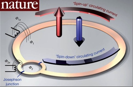
Fig.1 shows one of D-Wave’s superconducting flux qubits. It consists of two superconducting loops. Flux $\Phi_1$ plus a much smaller “bias flux” $\Phi_{1x}$ links loop 1. Likewise, $\Phi_2 + \Phi_{2x}$ links loop 2. The magnetic moment of loop 1 can point either up or down, and these two possibilities correspond to the two states $|0\rangle$ and $|1\rangle$ of the qubit.

Fig.2

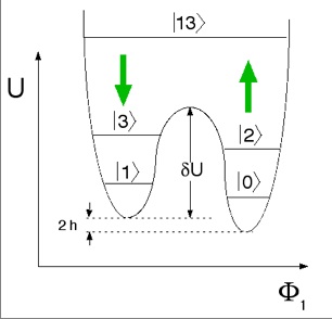
Fig.2 shows a potential energy curve for one of these qubit. The axes of the graph are energy $U$ versus flux $\Phi_1$ . A potential energy curve of this type is called a double-well potential. Let quantum state $|n\rangle$ occupy the discrete energy level $E_n$ for $n=0,1,2,...$ . The qubit can be localized in the right well, in states $|0\rangle$ and $|2\rangle$ , or in the left well in states $|1\rangle$ and $|3\rangle$ . The qubit can also occupy a state which is above the energy barrier and spreads over both wells (this is illustrated by state $|13\rangle$ in Fig.2.) At low temperatures, the qubit occupies, with very high probability, the two lowest states $|0\rangle$ and $|1\rangle$ (or a superposition of these two states).

The shape of the double-well potential of Fig.2 is characterized by two important parameters:

$\delta U$ is the height of the energy barrier. It can be changed by changing the flux bias $\Phi_{2x}$ .
$2h$ is the energy difference between the bottoms of the two wells. It can be changed by changing the flux bias $\Phi_{1x}$ . The spin of a qubit is proportional to its magnetic moment, which is proportional to $\Phi_1 + \Phi_{1x}$ . Furthermore, $\Phi_{1x}$ is proportional to $2h$ . Thus $2h$ can also be thought of as a spin bias. Note that $2h$ quantifies the symmetry breaking of the double-well potential.

For novices, it might help to think of the Y axis ( $U$ ) of the graph in Fig.2 as being the potential energy $mgz$ where $mg$ is the weight of an object and $z$ is how high the object is above the surface of the earth. You can think of the X axis ( $\Phi_1$ ) of the graph as the horizontal displacement of the object on the surface of the earth. Now imagine two buildings separated by a wall. Call the height of the wall $\delta U$ . The right building has two floors 0 and 2 and the left one has two floors 1 and 3. Both buildings also have a common floor 13. Floors that are higher than the wall, like floor 13, are connected and common to both buildings. Quantum mechanics allows a qubit to go from floor 0 to floor 1 or vice versa by walking through the wall (“tunneling”) instead of jumping over it. The bottoms of the buildings differ by $2h$ in their elevations. It’s possible to vary the height of the separating wall (this would change $\delta U$ ). It’s also possible to raise or lower one building with respect to the other (this would change $2h$ ).

The D-Wave paper reports on an experiment where $\delta U$ and $h$ both depend on time, varying approximately like step functions; that is, they rise from zero to a maximum value, doing this monotonically and fairly quickly. Let

$t_{delay}$ , the “delay time”, be the time at which $h(t)$ reaches half of its maximum value.
$t_{freeze}$ , the “freeze time”, be the time at which $\delta U(t)$ reaches half of its maximum value.

According to Suzanne Gildert, one could say that during the experiment, a snap-shot of the qubit was taken at each time $t_{delay}$ . This allowed D-wave to obtain a snap-shot of the qubit in flagrante delicto, i.e., right at the time $t_{freeze}$ at which it was performing “the act” (probably praying or brushing its teeth).

For times less than $t_{freeze}$ , $\delta U\approx 0$ , so the wall between the two buildings has approximately zero height. Thus, at such times the potential energy curve is parabolic-looking (as one gets for a harmonic oscillator), and the Hamiltonian $\cal H$ for all the qubits is approximately a trivial Hamiltonian, call it ${\cal H}_{trivial}$ .

For times greater than $t_{freeze}$ , $\delta U\approx \delta U_{max}$ , so the wall between the two buildings has maximum height. Thus, at such times the potential energy curve is a double-well, and the Hamiltonian $\cal H$ for all the qubits is a non-trivia Hamiltonian, call it ${\cal H}_{non-trivial}$ .

Fig.3

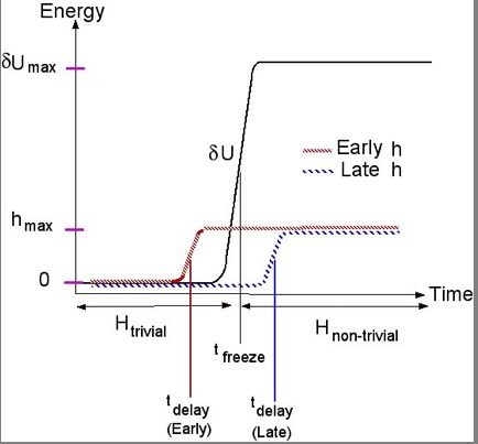
Fig.3 shows a qualitative graph of $\delta U(t)$ and $h(t)$ versus time. Actually, it shows two instances of $h(t)$ , one instance in which $t_{delay} < t_{freeze}$ so $t_{delay}$ is said to be “early”, and one instance in which $t_{delay} > t_{freeze}$ so $t_{delay}$ is said to be “late”. Note that $2h_{max}<<k_B T<<\delta U_{max}$ , where $k_B$ is Boltzmann's constant and $T$ is the temperature of the qubit.

In the EARLY case, $2h$ (=the difference in the elevations of the bottoms of the two buildings) is changed BEFORE the wall between the buildings is erected. In this case, if the qubit initially occupies floors 0 and 1 with equal probability, it sees NO WALL blocking its way, so it ends up moving with high probability (which depends on temperature) to floor 0, which is the lowest floor of the lowest of the two buildings, and that's how it is found at freeze time.

In the LATE case, $2h$ (=the difference in the elevations of the bottoms of the two buildings) is changed AFTER the wall between the buildings is erected. In this case, if the qubit initially occupies floors 0 and 1 with equal probability, it sees A HIGH WALL blocking its way, so it ends up not changing much, continuing to occupy floors 0 and 1 with equal probability, and that's how it is found at freeze time.

Fig.4

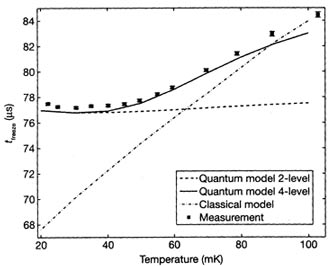
Fig.4 shows how $t_{freeze}$ changes with temperature for:
(1) a theoretical model that is quantum mechanical and assumes just two states $|0\rangle$ and $|1\rangle$
(2) a theoretical model that is quantum mechanical and assumes just four states $|0\rangle$ , $|1\rangle$ , $|2\rangle$ , $|3\rangle$
(3) a theoretical model that is classical,
(4) the data.

In Fig.4, the classical model (unlike the quantum models) gives a $t_{freeze}$ which depends linearly on temperature. This dependence can be explained as follows. $\delta U$ increases monotonically from zero to a value $\delta U_{max}>> k_B T$ . Thermal fluctuations can cause the qubit to jump over the wall, with probability $exp(\frac{-\delta U}{k_B T})$ , but this can only occur initially, while $\delta U$ is less than $k_B T$ . This suggests that the freezing occurs when $\delta U(t_{freeze}) \approx k_B T$ . Since $\delta U(t)$ varies linearly with time in the rising part of the curve, we expect $t_{freeze}$ to vary linearly with temperature.

Besides varying the $\delta U$ and $h$ of each qubit, the D-wave computer can also vary the coupling constant $J_{ab}$ between qubits $a$ and $b$ . Besides considering individual qubits, the paper also considers a chain of eight qubits coupled in such a way that a domain wall must form somewhere within the chain, with all spins on one side of the domain wall pointing in one direction and all spins on the other side pointing in the opposite direction. I won't go into the details of the 8 qubit experiment here. The bottom line is that, just as for the single qubit case, D-wave investigators observe for the 8 qubit chain a signature for quantum tunneling which fits well their quantum model and is very different from what one would get with any reasonable classical model.

In conclusion, Fig.4 and many other data plots given in the paper show quite conclusively that the D-Wave computer is doing quantum tunneling.

Separability Concerns

(This section deals with concerns about the separability of the density matrix describing the collection of 128 qubits in the D-wave computer. If you don’t know what a separable density matrix is, check out the appendix at the end of this blog post).

Some experts, while agreeing that the D-Wave computer is doing quantum tunneling, have pointed out that the D-wave machine uses a non-entangled density matrix, and that the (few) known quantum algorithms that give exponential speedups use entangled density matrices. However, this is not a very strong objection at the present time, because the claim

IF a quantum algorithm uses a non-entangled density matrix, THEN there are classical algorithms that can calculate the same thing as the quantum algorithm and just as fast (i.e., with the same time complexity)

has not been proven yet, and may not even be true. That this claim hasn’t been proven yet, has been emphasized (in more technical language) by Scott Aaronson in his blog post about the paper.

Even though the density matrix for the D-wave computer is separable, it is not totally classical, because it is non-diagonal in the physical basis, and it also exhibits quantum tunneling, which is a non-classical property. I find it hard to believe that a machine with the ability to do quantum tunneling cannot do some calculations faster (i.e., with a more favorable time-complexity) than any classical machine. I say this because a machine used for minimizing functions that takes advantage of quantum tunneling might be able to escape local minima on which a classical computer would get stuck.

Appendix: Separable Density Matrices

A two-part density matrix $\rho_{AB}$ is said to be separable iff it can be written as $\rho_{AB} = \sum_{i=1}^n w_i \rho^i_A\otimes \rho^i_B$ , where $n>0$ , where $w_1, w_2, \ldots, w_n$ are positive numbers which add up to one, and where, for all $i$ , $\ \rho^i_A$ and $\rho^i_B$ are density matrices. A non-separable density matrix is said to be entangled. For example, if $\rho_{AB}$ represents two qubits and acts on the vector space spanned by the states $\{|00\rangle, |01\rangle, |10\rangle, |11\rangle\}$ , then

$\rho_{AB} = \left[ \begin{array}{cccc}\frac{1}{2}&0&0& \frac{1}{2} \\ 0&0&0&0\\ 0&0&0&0\\ \frac{1}{2} &0&0&\frac{1}{2}\end{array}\right]$

is non-separable (i.e. entangled), whereas

$\rho_{AB} = \left[ \begin{array}{cccc}\frac{1}{2}&0&0&0\\ 0&0&0&0\\ 0&0&0&0\\ 0&0&0&\frac{1}{2}\end{array}\right]$

is separable (i.e., non-entangled).

If the system AB is classical, then $\rho_{AB}$ is diagonal. A diagonal $\rho_{AB}$ with diagonal elements $P(a,b)$ is separable iff $P(a,b)$ can be written in the form $P(a,b)= \sum_i P(a|i)P(b|i)P(i)$ . (Note that this condition is related to conditional independence. $P(a,b|i)$ is conditionally independent if $P(a,b|i)= P(a|i)P(b|i)$ ). All probability distributions $P(a,b)$ can be written in this form. Just write $P(a,b) = \sum_{a',b'} \delta_a^{a'} \delta_b^{b'}P(a',b')$ and set $i=(a',b')$ . Hence, all classical multi-part density matrices are separable.