Evolution of Quantum Computer Software – Pixar Analogy

Suppose commercial quantum computers are 10 years away. Should we wait until then to start developing QC software? No! The software must be ready at the same time as the hardware. It will take many years to invent and refine the software that powers QCs. A good analogy is Pixar. It took many years to invent and refine the computer graphics software that powers Pixar.

Pixar Timeline

• 1973- Dick Shoup begins writing SuperPaint. Shoup eventually fired from Xerox PARC for working on SuperPaint.
• 1974- Alvy Ray Smith collaborates with Shoup on Superpaint.
• 1975- Alex Schure, eccentric millionaire, hires Smith and Ed Catmull to work on graphics software (for Tubby the Tuba) at NYIT (New York Institute of Technology).
• 1979- George Lucas hires Smith and Catmull to start new computer division (Graphics Group) of LucasFilm
• 1984- John Lasseter, artistic genius, leaves Disney to join Graphics Group.
• 1986- Steve Jobs buys Graphics Group for $10 million.
• 2006- Disney acquires Pixar for $7.4 billion

Moral for investors: Gathering and nurturing a cohesive talent pool for a worthy endeavor takes time and patience, but it pays off handsomely.

Taxonomy of Existing Quantum Computer Software

(Updated on Aug 31, 2009 to include QuSAnn and MultiplexorExpander)

It’s important to classify existing quantum computer software, to see what we have and what we are missing. I like to classify such software as follows. Define the following binary variables: T = text (programming language) input, V = visual (gui) input, N = numeric input. (these variables are not to be confused with Temperature, Volume, and Number by the inveterate thermodynamicist). Ideal software like WinBugs has (T,V,N)=(1,1,1)

• quantum computer simulators:
  • exact: Quantum Fog (T,V,N)=(0,1,1)
  • approximate
    • Monte Carlo (quantum circuit samplers): quantum WinBugs (doesn’t exist yet)
    • variational
• quantum compilers (U input, where U = unitary matrix)
  • general-U compiler: Qubiter (T,V,N)=(0,0,1)
  • special-U compiler: QuanSuite (T,V,N)=(0,0,1)
• quantum circuit generators (“code generators”): (don’t have explicit U input as compilers do)
  • uses standard language (C, C++, etc.): QuSAnn (T,V,N)=(1,0,0)
  • uses new “quantum language”: (T,V,N)=(1,0,0)
• error correction add-ons
• code translators: Multiplexor Expander
• other tools
  • drawing: Q-circuit
  • numeric: M-fun

The names in italics are computer programs that I have written. Surprisingly, I am not the center of the universe; many others have written quantum computer programs too. Here is Quantiki’s list of such software. Their list classifies the programs by the language they are written in. It calls all programs “simulators”, which is less precise than the above taxonomy.

An Elevator Pitch for Quantum Computers

We live in an era of large data sets. To analyze those large data sets, we use Monte Carlo methods, and such methods require good random number generation. Quantum Mechanics provides perfect random number generation. So we want a computing device that harnesses the random nature of quantum mechanics to the utmost. Sounds like a job description for a quantum computer. Here is a flow chart of this argument.

Mathematicians, you don’t scare me

My Ph.D. is in theoretical physics, so naturally, I have taken a fair number of “rigorous” math courses (theorem, proof, theorem, proof, …on and on, like an Iowa corn field). I think it’s important, although not easy, for a theoretical physicist not to be intimidated by rigorous math.

One thing that I’ve noticed from reading their books is that mathematicians have a fetish for inequalities. Their proofs often follow easily from an inequality, but only God, and mathematicians, know where that inequality came from. Sure, mathematicians will give you a proof of an inequality, but the proof is often as mysterious as the inequality itself. Providing motivation for what they are saying is not the strong suit of mathematicians.

Then one day I realized, hey, physicists have a fetish for approximations. And although mathematicians wrinkle their noses every time they see a physicist do an approximation, and physicists wrinkle their noses every time they see a mathematician write down yet another inequality, they are essentially doing the same thing.

As a trivial example, take the Cauchy-Schwarz inequality for two vectors. All it’s saying is that when the two vectors are nearly parallel, you can approximate their dot product by the product of their lengths. Mathematicians, you don’t fool me, you love approximations too. Come out of the closet!

It’s true, inequalities are more powerful than approximations; they’re like approximations on steroids. But I bet most inequalities were initially conceived as humble approximations, and then someone came along and said, What Ho!, we can promote this into an inequality, and get a math paper out of it. Goes the other way too. Often, when we are doing a back of the envelope estimate, we demote an inequality into an approximation.

Bell’s Inequalities for Bayesian Statisticians

My Ph.D. is in physics, so the famous Bell’s Inequalities of quantum mechanics have been hammered into my mind by the educational system since an early age. But maybe I can pique the interest of Bayesian statisticians with little or no exposure to “the other probability theory”, “the other red meat”, i.e., quantum mechanics, by introducing Bell’s inequalities in a language familiar to them, that of Bayesian networks. Yes, indeedy, you heard right. Although seldom done, Bell’s inequalities can be explained simply and intuitively using the language of Bayesian networks, as follows.

Henceforth, I will underline letters that stand for random variables.

A simple Bayesian “model” might have a “parameter” such that and i.i.d. “data” such that . This can be represented by the Bayesian net shown in Fig.1. The data is observed (evidence) and the parameter is inferred from this.

Fig.1

Now consider two point particles that start off at the same point, and then fly apart without interacting with anything else. Let’s assume that both particles are spin-1/2 fermions (like electrons, protons and neutrons), and that they start off in a state of zero angular momentum. In a “Local Realistic” theory, this situation can be represented by the classical Bayesian net shown in Fig.2.

Fig.2

In Fig.2, node represents the “hidden variables”. For , node represents the outcome of a spin measurement performed on particle . represents the measurement axis. Node may assume two possible states, + or −, depending on whether the measurement finds the spin to be pointing up or down along the axis . For example, if a measurement of the spin of particle 1 along the A axis yields “up”.

It is convenient to define the following probability functions

where .

Fig.2 implies the following equation:

The assumption that the particles start off in a state of zero angular momentum
means that

where , and is the opposite of , so and .

It can be shown (see Ref.2 for a proof) that Eqs.(5) and (6) imply that

and the 5 other inequalities one gets by permuting the symbols A,B and C.

Assume axes A,B and C are coplanar and that . Also let x = +, y = − and z = + in Eq.(7). Quantum mechanics gives an expression for as a function of . Combining Eq.(7) and the expression given by quantum mechanics for yields:

which is false for , for example.

Thus, quantum mechanics and Local Realism are incompatible. Quantum mechanics tells us that if you measure the spin of particle 1 along the A axis and the spin of 2 along C, where angle(A, C) = 270 degs., and if you do this many times, you will get a probability that is greater than that predicted by Local Realism. Somehow the particles know more about each other than one would have expected from Local Realism alone.

This blog post is an abridged version of Ref.2. Look in there for more details.

References:

1. here. Wikipedia article on Bell’s inequalities. Explains them in the conventional way, in terms of expected values, without alluding to Bayesian networks
2. here. An excerpt (pages 43-49) from QFogLibOfEssays.pdf, which is part of the Quantum Fog documentation

Quantum Circuits in ASCII

I think quantum computing is the wave of the future. That’s why my quantum computer software QuanSuite uses futuristic, advanced computer graphics techniques like ASCII art. For example, behold how QuanSuite renders a 4-qubit quantum Fourier transform circuit:

In these types of diagrams, time points downward, and

• “|” stands for a qubit wire (connecting the same qubit at two successive times)
• “–” stands for a piece of a connector between two different qubits
• “H” stands for a Hadamard gate
• “@” or “0” stands for the 2 possible kinds of control qubits of a controlled gate
• “X” stands for the target qubit of a controlled gate.

, etc.

A simple CNOT looks like this: |   X---@    |

A swap looks like this: <---+--->   |

Being Bayesian in Java

I’ve written software for quantum computers in several computer languages. Most recently, I wrote QuanSuite in Java. I was able to learn Java very quickly, thanks to the wonderful textbook I learned it from. I am referring to Prof. Daniel Liang’s “Introduction to Java Programming, Comprehensive Version”. The book costs about a hundred bucks. But for that you get more than 1300 pages. I like to “read” computer programming books by reading the code examples only. Only if I don’t understand something do I read the text. This technique works better with some books than with others. It works great with Liang’s book. Examples and definitions are clearly highlighted in this book. The book is very well edited. I found very few errors in it, which is remarkable for a 1300 page book. Prof. Liang’s website has some useful resources. I like to use the Eclipse development environment (freeware).

Is there any Bayesian software written in Java? There was a recent blog post about this in Prof. Andrew Gelman’s blog. (Gelman is a noted professor in Statistics and Political Science at Columbia University. He has written several books on Bayesian Statistics).

Quantum WinBugs in Java?

WinBugs on Trees

My romance with WinBugs continues. Recently, I’ve been avidly reading books on Bayesian statistics so I can understand her better. WinBugs knows quite a lot about Bayesian statistics, so I can whisper questions to her on this subject at night. I recommend that you read her well written manual. Among WinBugs nice qualities is a tool (DoodleBugs) that allows you to draw Bayesian networks, and then to turn them into text code. Cute. Here is how she likes to speak of trees…she is such an artist. Suppose you are interested in the following tree graph.

WinBugs would draw this as follows:

These are called “plates”. They allow you to picture arrays of random variables succinctly. (Statisticians are very interested in many, identically distributed random variables (samples), which are conveniently grouped into arrays.) In the plate representation, it’s as if you are looking at a book, and in each page of that book is another tiny book, and in each page of the tiny book is another even tinier book; this, ad infinitum if need be. WinBugs would re-express this “plates” figure as poetry (i.e., code) as follows:

Nice! Her coding style is clear and succinct. What a woman!

Winsome WinBugs

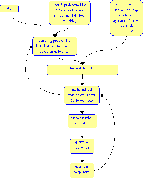
Lately, I’ve been reading everything I can lay my hands on that has to do with the use of Monte Carlo methods in mathematical statistics, and, especially, applications of this to sampling of Bayesian networks. There are books and software galore on the subject. Hard to sift through it all. So here is a recommendation. A truly beautiful program that does sampling of Bayesian networks is WinBugs. I found the tutorial Getting started with WinBUGS (by James B. Elsner and Thomas H. Jagger, Department of Geography, Florida State University) an excellent first tryst with this software beauty.