Also available on the web as HTML (takes a few seconds to open because it’s a 30 MB single file) (IMPORTANT: Open the HTML in an INCOGNITO tab. If you open the HTML in a regular tab, you are likely to get an old version residing in cache.) https://www.ar-tiste.com/bayesuvius.html
21-year-old activist Mario Savio gives a passionate speech at the University of California, Berkeley on December 2, 1964. He was arrested, along with 800 others. Hoover’s FBI was terrified of this speech.
“Without experiment, I am nothing”. –Michael Faraday
Causal AI and Causal Inference allows us to add to AI the heretofore missing features from AI, of experimentation (a.k.a. intervention) and the scientific method.
I write AI software (for detecting causes of diseases, not for killing people). I am very disgusted because ALL the famous people that have been debating, prior to the Lavender and Nimbus revelations, whether AI is safe or an existential threat to humanity, have become totally silent after the revelations surfaced. It shows that these people, just like the members of Congress or our psychopath president, Genocide Joe, have no moral backbone and are easily bought. I just can’t think of a more horrific use of AI than to generate target list of families to assassinate at night, while they sleep in their homes.
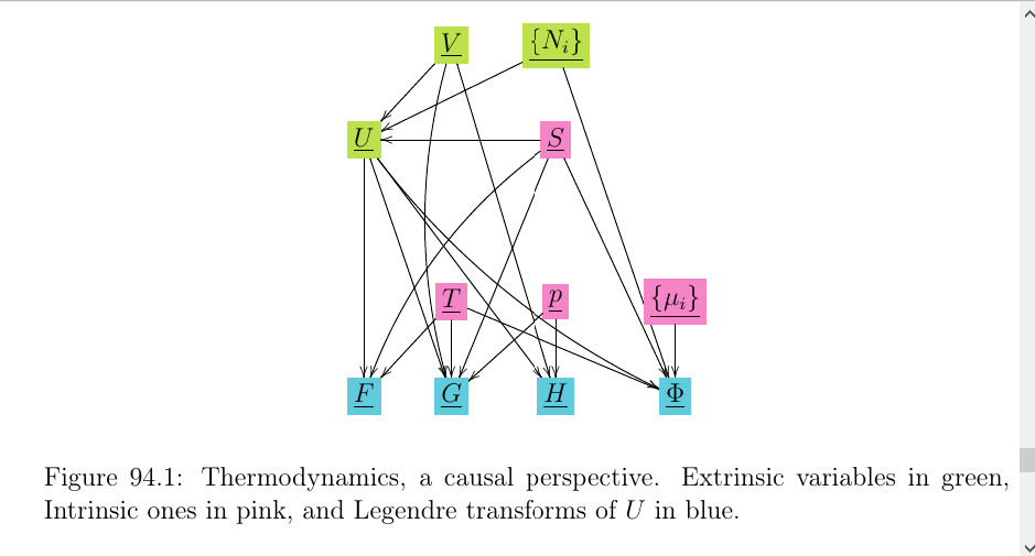
Just finished a short (2 pages) chapter called “Thermodynamics, a Causal Perspective” for my free, open source book Bayesuvius. (880 pages). It’s no big deal, but was fun to write. I got the idea out of the blue this morning, and by the end of the day, viola. The chapter discusses the following Bayesian Network
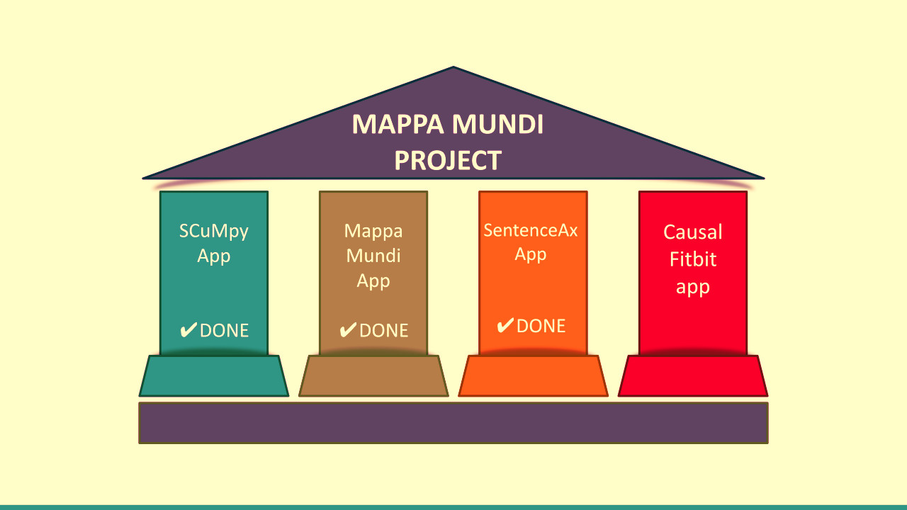
Software is never finished. There are a few details and some known bugs that still need fixing, but I believe the current version of MMP tackles successfully every major obstacle to its goal. And what is that goal, you ask? This
When dealing with causal DAGs and Bayesian Networks (bnets), it is often necessary to store them for future reuse. For instance, my Mappa Mundi software stores bnets for future reuse. It does so continuously, as they are learned by the AI. The bnets are stored in a directory that I call a DAG atlas. The current version of Mappa Mundi stores the bnets as a pickle file of some Python classes. But future versions of Mappa Mundi will store them in human readable form, and in a format that is standardized, namely in YAML.
The purpose of this blog post is to announce that my free, open source book Bayesuvius (825 pgs.) now contains a short chapter explaining how, in the future, Mappa Mundi will store bnets in YAML. Here is an example.
graph0:
  nodes:
    - id: A
      label: Node A
      values:
        - 0
        - 1
      parents: None
      probabilities: [0.3, 0.7]
    - id: B
      label: Node B
      values:
        - 0
        - 1
      parents:
        -A
      probabilities: [[0.8, 0.2], [0.6, 0.4]]
    - id: C
      label: Node C
      values:
        - 0
        - 1
      parents:
        - A
      probabilities: [[0.8, 0.2], [0.6, 0.4]]
    - id: D
      label: Node D
      values:
        - 0
        - 1
      parents:
        - B
        - C
      probabilities: [[0.9, 0.1], [0.3, 0.7], [0.5, 0.5], [0.4, 0.6]]
  edge_gains:
    (A, B): 3 # arrow from A to B has gain 3
    (A, C): 5
    (B, D): -6
    (C, D): 3
Why YAML?
There are infinitely many ways of storing a bnet. The reasons why we propose using the YAML language is that it is a popular, standardized, human readable, and fairly succinct language.
The configuration information of a software app, and the data exchanged between apps, is often stored in a YAML data structure.
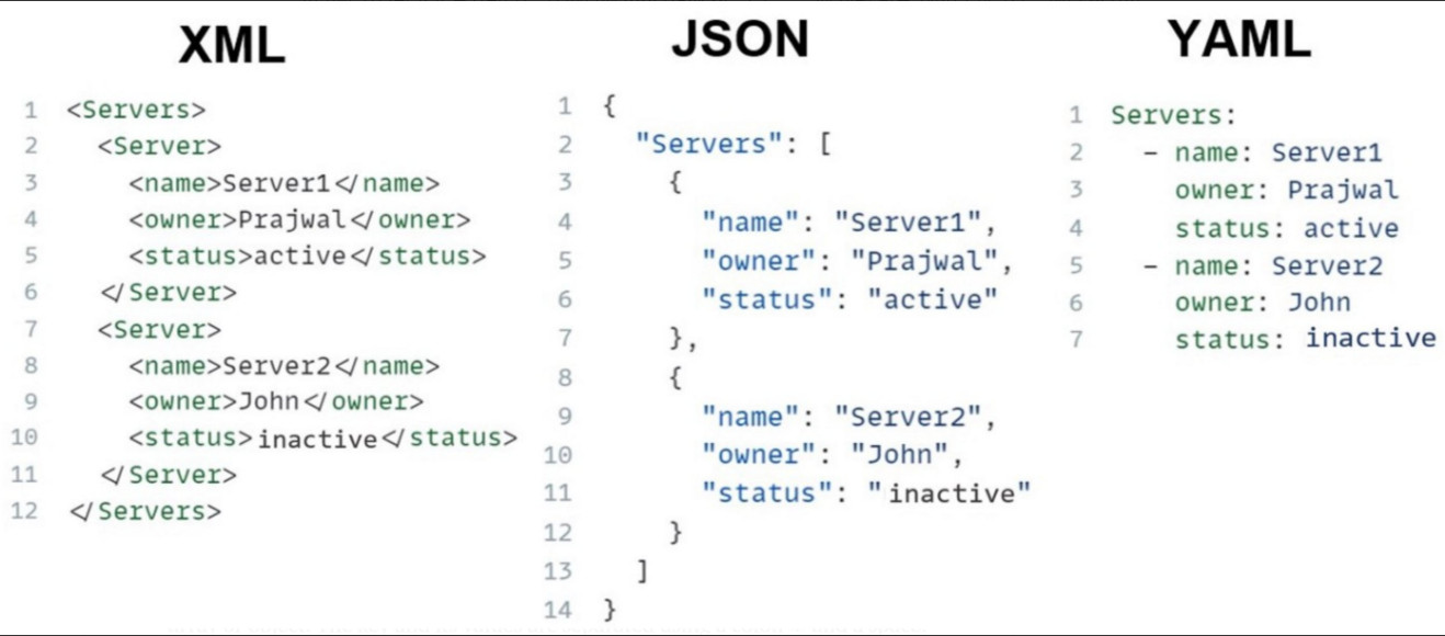
YAML is a human-readable data serialization language. XML and JSON are too. As illustrated by the figure below, for simple data structures, one can translate a data structure from one of those languages to the other 2. But note that YAML is the most succinct of the 3 languages. So in this blog post, we speak only about YAML, although our format could be easily translated to XML or JSON
Boring, Bob. Who cares about storing bnets in YAML?
Okay, you got me there. Very few people do. I do though, for the following reasons.
I am not claiming that this blog post presents a significant advancement in causal inference. On the contrary. I think this blog post is a boring, pedestrian but necessary practical move towards standardization in the CI field.
I believe that in the future, all AIs will carry a DAG atlas. The advantages of a DAG atlas are just too important and numerous to ignore:
A casual DAG atlas carries causal DAGs. DAGs are necessary for distinguishing between correlation and causation. AI’s that don’t distinguish between correlation and causation will be superstitious.
An AI with a DAG atlas will be very explainable,
An AI with a DAG atlas will be easy to transport between software apps and between usecases
An AI with a DAG atlas will be easy to align (just remove a few unwanted DAGs from the DAG atlas)
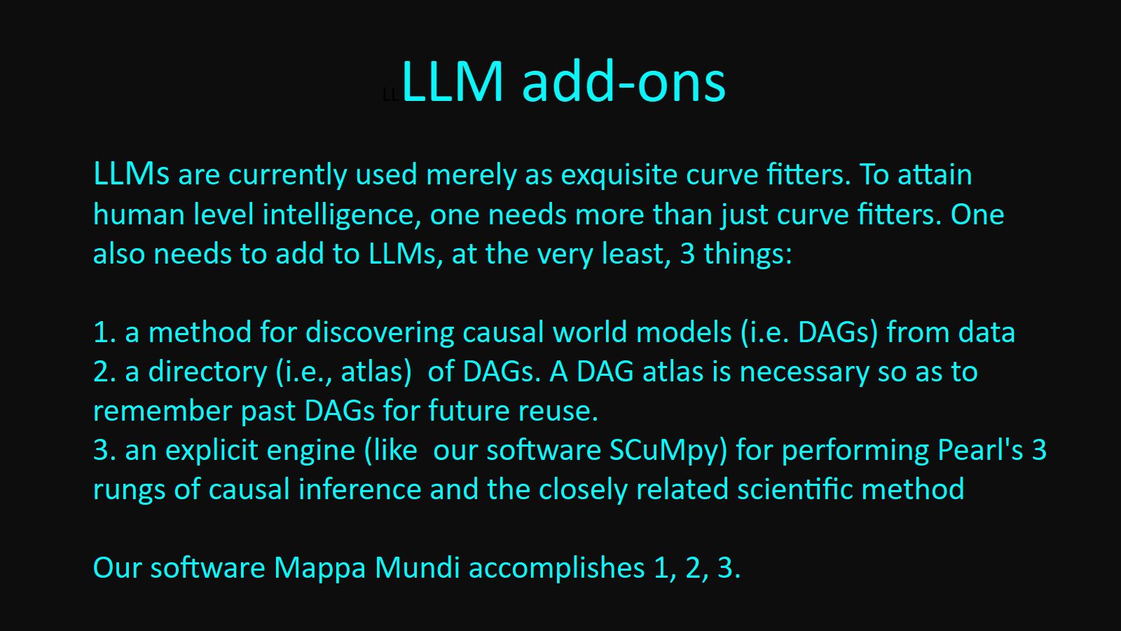
A DAG atlas can be added very naturally to an out-of-the-box LLM as an add-on. This is what Mappa Mundi does. Some people talk about adding causal inference to Reinforcement Learning (RL). Two serious problems with current causal RL are
current schemes for doing causal RL don’t use a DAG atlas, so advantages 1, 2, 3, 4 given above are lost.
most current schemes for doing causal RL (for example, Bengio’s flow networks) do not use an LLM. They use their own NNs that are not based on text, so no LLM. Those that do use LLMs, use it very indirectly. The marriage between RL and LLM is not a very close one, like that of Trump and Melania.
Contrast this with Mappa Mundi. Mappa Mundi uses a DAG atlas and uses LLMs twice: first it uses a BERT fine tuning to do sentence splitting, and then it uses sBERT to do sentence similarity. How is that for a perfect marriage, twice blessed!
The Openie6 (O6) software splits complex or compound sentences into simple ones. Simple sentences are essentially the same as the triples (subject, relationship, object) which, when visualized as a directed or undirected graph, is called a “knowledge graph”. Sentence splitting is also a necessary step in doing DAG extraction from text (DEFT), as is done by my software Mappa Mundi.
My open source software SentenceAx (Sax) is a complete re-write of the O6 software.
SentenceAx is a fine-tuning of BERT written with PyTorch and Lightning.
The purpose of this blog post is to announce that Sax has been fully trained for the first time. Knut Jägersberg generously provided some initial assistance, but encountered some bugs in the training. After I fixed those, Nick Marino took over as Sax Model Trainer and Tamer. He generously offered to train Sax on his home gaming computer which has a GPU (an NVIDIA RTX 3080). I have no GPU on my computer so this was a God Send. He has done a full Sax training run that seems solid to me. It took 13 hours and the weights file is about 1.2GB before zipping. I prepared a google Colab Jupyter notebook so you can look at the TensorBoard logs without needing to download them. Here it is. If you want to expand all 7 plots at once and view them all in a single pane, do a search for _* (underscore, star).
The Openie6 (O6) software splits complex or compound sentences into simple ones. Simple sentences are essentially the same as the triples (subject, relationship, object) which, when visualized as a directed or undirected graph, is called a “knowledge graph”. Sentence splitting is a necessary step in doing DAG extraction from text (DEFT), as is done by my software Mappa Mundi.
My open source software SentenceAx (Sax) is a complete re-write of the O6 software. Sax is 95% identical algorithmically to O6, but I have rewritten it in what I hope is a friendlier form.
The purpose of this blog post is to announce that my free, open source book Bayesuvius (818 pages) now contains a chapter explaining SentenceAx in terms of Causal DAGs. I’ve excerpted the SentenceAx chapter here, in case you want to download only that chapter instead of the whole book.
Here is the diagram provided by the creators of O6 to explain the O6 software. This diagram is very typical of the diagrams currently being used by AI workers to describe Deep Learning/NN/Transformers.
And here is how I describe, using causal DAGs, exactly the same algorithm and transformer model. Quite a difference!
How does Sax fit into the AI universe? A small asteroid in a Universe with 1E23 stars.
Sax is a fine tuning of the BERT model. What this means in the language of Bayesian Networks is simply that Sax uses BERT as a prior probability.
“vanilla transformer network” is the popular name given to the NN model proposed in the highly influential 2017 paper entitled “Attention is all you need”. This paper introduced the terms “Transformer Networks” (tranets) and “Attention” into the AI vernacular. I recently discussed the vanilla tranet from a causal DAG point of view here.
The BERT model was published a year after the “Attention is all you need paper”. The BERT model is simply the encoder half of the vanilla tranet. As far as LLMs are concerned, BERT, which contains 1E8/3E8 parameters in its base/large flavors, is a small LLM. The big boys LLMs nowadays contain 5E11 parameters! An increase in size by a factor of 1E3 in only 6 years!
Both Joshua Bengio and Daphne Koller, two legendary figures of AI, believe distinguishing between correlation and causation, and being able to do experiments (interventions) to determine causation, are a necessary next step in AI. Yann LeCun disagrees. Yann’s theory of “Objective Driven AI” (ODAI) doesn’t do this. Yann has been working on ODAI for 9 years and failing. Watch this Davos panel discussion where Daphne Koller totally destroys Yann’s crackpot flat earth theory of AI. Amazing discussion: Koller flew a hundred feet above the other members of the panel, like an eagle observing field mice on the ground.
The purpose of this blog post is to announce that my free, open source book Bayesuvius (807 pages) now contains a chapter explaining Transformer Networks (tranets) as Causal DAGs. I’ve excerpted the tranet chapter here, in case you want to download only that chapter instead of the whole book.
There are quite a few top quality blog post on the internet explaining Transformer Networks and Attention. Each one is excellent in its own way, and I had the pleasure to read many of them to learn about this topic. My only claim to fame is that in this chapter, I commit blasphemy by calling them causal DAGs.